From Reinforcement Gamer to Reinforcement Trader
Use reinforcement learning to train an algorithmic trader to trade stocks automatically
Introduction
This is the second part of from reinforcement gamer to reinforcement trader. It shares a lot of resemblance to the notebook of part one. As illustrated in the figure below, investing bears a clear resemblance to game playing. In fact, some good poke players, such as Edward Thorp, also stand out in the stock markets.
Reinforcement Learning (RL) is a branch of machine learning that enables an agent to reach an objective by learning how to interact with an environment. Of all the machine learning techniques, it is considered most similar to human learning by taking actions in the real world and observing the consequences. In particular, RL resembles how a novice trader becomes a legendary trader in the stock market by learning from her own trading experience.
RL has been applied to stock trading and portfolio management. On the trading front, Xiong, Zhuoran, et al (2018) explore the stock market and Zhang, et al (2020) trade the futures market. On the portfolio management front, Jiang, Z., Xu, D., & Liang, J. (2017) investigate the asset allocations among Bitcoin and 11 other digital assets. Liang, Z., Chen, H., Zhu, J., Jiang, K., & Li, Y. (2018). compare the performance of DDPG, PPO, and PG in China stock market. Refer here for more references.
In this post, we will train an agent to trade in stock markets. We first introduce the OpenAI Gym environment, then use DQN (Deep Q-Networks) to train the trading agent, and evaluate her trading performance. The full notebook with embedded videos is located here on GitHub.
Trading Environment
Below is a typical RL environment. In the context of stock trading, the agent is a stock trader. Her action can be to buy, sell, or hold on (do nothing) a stock. The Environment is the stock market, and observation includes the stock prices, technical indicators, and market news, among other useful information. The reward can be the cash reward or some sort of risk-adjusted objectives.

Let’s take one step forward to see how the environment works.
o1 = eval_qt_env.reset()
action = 1
o2, reward, done, info = eval_qt_env.step(action)
o1.shape, o2.shape((10, 14), (10, 14))
It indicates that the observation has fourteen features, including daily OHLCV, eight technical indicators, and NAV (net asset value). The lookback window is 10 days or two weeks.
eval_qt_env._df_exch[idx0:idx1]                      SPY
2012-01-03 15:59:59   127.500000
2012-01-04 15:59:59   127.699997
2012-01-05 15:59:59   128.039993
Here is how the trader and stock market interact with each other. At the end of 2012–01–03, if action is one or she is all in SPY, then she buys $100,000/$127.50 or 784 shares, incurring a commission of 784x$127.50x0.0001=$9.996, and the remaining cash is $100,000–784x$127.5–$9.996=$30.
Then the market moves to 2012–01–04, and SPY price goes up to $127.70. Her 784 shares are now worth 784x$127.70, and NAV including cash becomes 784x$127.70+$30=$100,146.80. The reward is $146.80.

Training A Trader
Before we train the trader, let’s see how a novice spontaneous trader looks like, as a comparison.
random_policy = random_tf_policy.RandomTFPolicy(train_env.time_step_spec(), train_env.action_spec())create_policy_eval_video(train_env, random_policy, "random-agent", num_episodes=1)

Above it shows a spontaneous trader’s random trading behaviour. The upper half is the SPY price chart along with red buy and green sell marks. The lower half is her NAV or total asset value. The trading window is from 2011–04 to 2012–04. Note that due to random trading windows and random trading actions, re-run the notebook each time will generate a slightly different video.
Now it’s time to train a sophisticated trader through DQN. DQN became popular in 2013 after DeepMind published research papers showing an AI system that achieves human-level performance when playing Atari games. It uses a neural network to approximate the q-function in Q-Learning. It also introduces experience replay buffer and freezing target network to improve performance.
Fortunately, we don’t have to recreate the wheel. There are a couple of RL libraries available to use out-of-box, such as Tensorforce, Ray’s RLLib, OpenAI’s Baselines, Intel’s Coach, Keras-RL, and TF-Agents. Here we follow the TF-Agents online tutorial.
fc_layer_params = (100, 50)action_tensor_spec = tensor_spec.from_spec(train_env.action_spec())num_actions = action_tensor_spec.maximum - action_tensor_spec.minimum + 1def dense_layer(num_units):return tf.keras.layers.Dense(num_units,activation=tf.keras.activations.relu,kernel_initializer=tf.keras.initializers.VarianceScaling(scale=2.0, mode='fan_in', distribution='truncated_normal'))
dense_layers = [dense_layer(num_units) for num_units in fc_layer_params]
q_values_layer = tf.keras.layers.Dense(num_actions,activation=None,kernel_initializer=tf.keras.initializers.RandomUniform(minval=-0.03, maxval=0.03),bias_initializer=tf.keras.initializers.Constant(-0.2))q_net = sequential.Sequential(dense_layers + [q_values_layer])
The q-network is a three-layer fully-connected deep neural network, which consists of a sequence of dense layers followed by a dense layer with num_actions units to generate one q_value per available action as its output. The input observation has 10 days x 14 features, flattened to a shape 140 tensor. The first layer has 100 neurons. Therefore, it requires 140×100+100=14,100 parameters. The second layer has 50 neurons, implying 100×50+50=5,050 parameters. The output layer is a binary decision of either buy or sell, which needs 50×2+2=102 parameters.
agent = dqn_agent.DqnAgent(train_env.time_step_spec(),train_env.action_spec(),q_network=q_net,optimizer=optimizer,td_errors_loss_fn=common.element_wise_squared_loss,train_step_counter=train_step_counter)
The agent is equipped with the Adam optimizer, squared loss function, and the q-network. It takes around one day on free-layer Google Colab to train one million episodes, so a trained agent is provided here on Github if you want to have a preview of how it trades. Hiring that trader (by wget, unzip, and re-load) should give the same performance matrix as below.
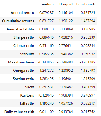
The reinforcement trader outperforms random spontaneous trader. She delivers slightly less annual return than buy-and-hold (11.6% vs 12.17%) but provides better risk-adjusted measures (Sharpe 1.028 vs 0.955).
Observing how she trades, it turns out she correctly recognizes the bull market between 2013 and 2015 by simply holding a long position, then starts adjusting her positions since the second half of 2015.
Conclusion
This post studies empirically reinforcement learning in stock trading. It builds an OpenAI trading environment and then trains a DQN agent using the TF-Agents library. The trained trader performs much better than the naive spontaneous trader, and also outperforms buy-and-hold in the risk-adjusted sense.
In the next post, we will explore the multi-period portfolio management strategies, where the portfolio adjustment actions are continuous so PPO is used to train the portfolio manager.
